Difference-in-differences in a repeated cross-sample

Author

Ville Voutilainen

See the did repo for updated notebooks and source code.

Background

Assume we are measuring observations for a repeated cross-sample of \(N=600\) individuals (e.g., customers at a marketing platform, new bank loans, etc.) at time points \(t = 0, 1, \cdots 19\). There are two distinguished groups of individuals (\(j=C,T\)), for example, from two different areas.

Imagine that in one of the areas there is a one-off intervention (e.g., a government stimulus package) taking place between time points 2 and 3 that might affect a feature of interest (“outcome”) of the individuals (e.g., time spent on the site, pricing of the loans). We are interested in the treatment effect of the intervention on the outcome.

Data-generating process

We consider a data-generating process (DGP) of the following form:

\[ \begin{equation*} Y_{ijt}^0 = \gamma_j + \xi_t + \lambda_t X_{ijt} + \epsilon_{it} \end{equation*} \]

where

  • \(\gamma_j\) is a group-specific, time-invariant effect;
  • \(\xi_t\) is a time-specific effect (affecting all individuals/groups the same way);
  • \(X_{ijt}\) is an individual-group-time-specific effect. \(\lambda_t\) denotes the (possibly time-varying) effect of \(X_{ijt}\);
  • \(\epsilon_{it}\) denote individual-and-time-specific idiosyncrasies.

The effect of the intervention is modeled as an additive effect:

\[ \begin{equation*} Y_{ijt}^1 = Y_{ijt}^0 + \tau_{jt} , \end{equation*} \]

where \(\tau_{jt}\) is the (possibly group- and time-dependend) treatment effect. We allow for either a constant or a linearly evolving \(\tau_{jt}\). See the notebook did_simulated_datasets.ipynb in the did repo for more in-depth explanation of the DGP.

Notice that, in reality, the true data-generating process is unknown to the researcher! Here we use simulated data (properties of which we know) to help us understand the properties of our research design and regression models. As advocated by Gelman, Hill, and Vehtari (2020, section 5.5), fake-data simulation is a “way of life” to evaluate the statistical methods.

Research design

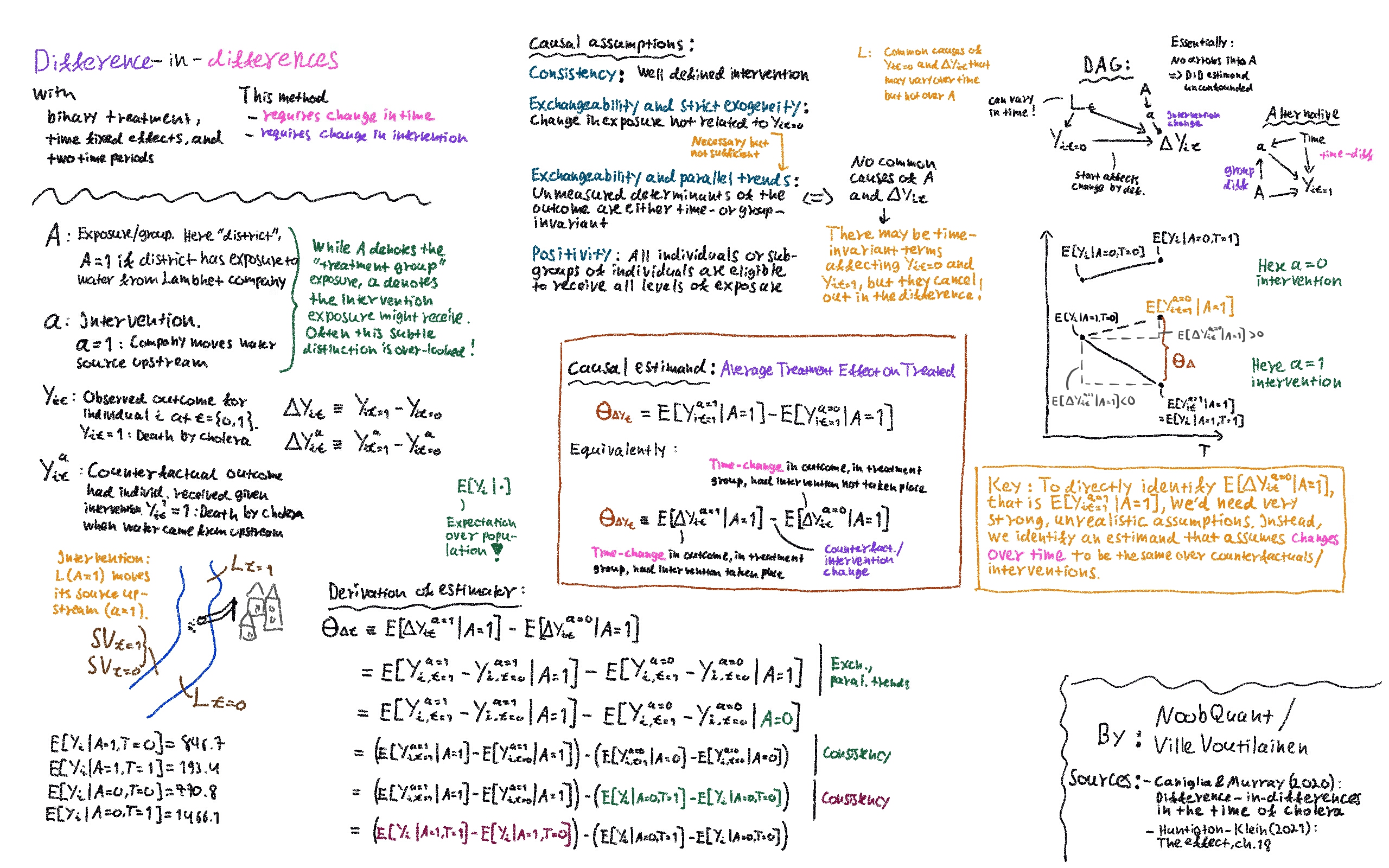
Assume we are interested in the average treatment effect on the treated (ATT). That is, we would like to know how much the intervention affected (on average) the outcome for individuals in the treated group. We can write this estimand in mathematical form using potential outcome notation:

\[ \begin{equation*} \theta = E[Y_{i}^1(post) - Y_{i}^0(post) \ | \ j=T] \end{equation*} \]

where

  • \(Y_{i}^d(post)\) denotes the potential outcome of an individual \(i\) at post-period under treatment \(D=d\);
  • expectation operator is to be understood to average over individuals \(i\) (and over \(t\) since our estimation is done at the level of pre/post periods instead of individual time points);
  • the post-period consist of time points 10-19 (and the pre-period of time points 0-9).

Some references for DiD:

Technical details for running the notebook

Used conda environment is dev2023a from here. Additionally installed packages:

  • r-dagitty via conda/mamba: mamba install r-dagitty. Also installs dependencies.

Imports

Code
# Python dependencies
import warnings
warnings.filterwarnings('ignore')
import numpy as np
import pandas as pd
import matplotlib.pyplot as plt
import statsmodels.formula.api as smf
np.random.seed(1337)

# Local helpers
from did_helpers import(
    simulate_did_data,
    plot_repcrossec_data,
    parallel_trends_plot,
    dynamic_did_plot,
)

# R interface
import rpy2
%load_ext rpy2.ipython
Code
%%R
library(dagitty)

Helper functions

Code
def prepare_static_regression_frame(data):

    df = data["observed"].copy()
    
    # Possible interaction between time and X if X present
    if "X" in df.columns:
        df["X_time"] = df["X"] * df["t"]
    
    # Code categories as dummies
    df["dummy_period"] = df["time_group"].map({
        "before": 0,
        "post": 1,
    })
    df["dummy_group"] = df["treatment_group"].map({
        "control": 0,
        "treatment": 1,
    })
    df["dummy_group_x_period"] = df["dummy_period"] * df["dummy_group"]
    
    # Time points as categorical/str
    df["t"] = df["t"].astype(str)

    return df

def prepare_dynamic_regression_frame(data):

    df = data["observed"].copy()
    param_last_pre_timepoint = data["params"]["param_last_pre_timepoint"]
    
    # Variable measuring periods to first treatment time 
    df["time_to_treat"] = (
        df["t"]
        .sub(param_last_pre_timepoint+1)
        .astype('int')
    )

    # We want to create "treatment" dummies from the time_to_treat column such that the kth dummy
    # obtains value 1 for a given observation if the period of the observation equals k.

    # To this end, first set time_to_treat cor control observations to 0, as the treatment
    # dummy values need to be zero for them.
    df.loc[df["treatment_group"]=="control", "time_to_treat"] = 0

    # Now create the "dynamic" dummies from time_to_treat. Drop out the last time point before treatment
    # manually to avoid multicolinearity problems (this sets the last time point before treatment as a
    # reference) point.
    df = (
        pd.get_dummies(
            df,
            columns=["time_to_treat"],
            prefix="dummy_group_x_period",
            drop_first=False
        )
        .rename(columns=lambda x: x.replace('-', 'm'))
        .drop(columns="dummy_group_x_period_m1")
    )

    # Time points as categorical/str
    df["t"] = df["t"].astype(str)

    return df

Classical two-period DiD

We start with a specification where in the true data generating process there is no effect \(\lambda_t X_{ijt}\).

Simulate and plot data

Code
# Simulate
data_1 = simulate_did_data(
    param_datasettype="repeated cross-section",
    param_no_t=20,
    param_N=1000,
    param_gamma_c=4,
    param_gamma_t=1,
)

# Plot
plot_repcrossec_data(data_1)
Realized control pre-period mean 8.509
Realized control post-period mean 18.498
Realized treated pre-period mean 5.497
Realized treated post-period mean 13.491
Counterfactual (unobserved) treatment post-period mean 15.491
Counterfactual (naively estimated) treated post-period mean 15.486
Naive DiD-estimate -1.995

Research design

Represent the research design as a directed acyclical graph. Explanation of the arrows:

  • Intervention affects individuals in the treated group but only in the post period. Hence, there is an arrow \(D_{it} \rightarrow Y_{i, post}\).
  • Time fixed effects \(\xi_t\) affect outcomes in each time point of pre and post periods (\(\xi_t \rightarrow Y_{i,pre}\) and \(\xi_t \rightarrow Y_{i,post}\)).
  • \(Y_{i,pre}\) and \(Y_{i,post}\) trivially affect their difference, hence the arrows \(Y_{i,pre} \rightarrow Y_{i,post} - Y_{i,pre}\) and $ Y_{i,post} Y_{i,post} - Y_{i,pre}$.
  • Group-level effect \(\gamma_j\) acts as a confounder in cross-sectional dimension: it causes* the treatment assignment to treatment/control groups (\(\gamma_j \rightarrow D_{it}\)) as well as the outcome in each time point of pre and post periods (\(\gamma_j \rightarrow Y_{i,pre}\) and \(\gamma_j \rightarrow Y_{i,post}\)). Due to this, we could not simply compare \(E[Y_{it} | j=T]\). The DiD estimator automatically controls for time-invariant, group specific effects via the double differencing. Hence, as Zeldow & Hatfield (2021) define it, \(\gamma_j\) does not constitute a confounder in a multi-period DiD setting. In order for a time-invariant group-specific covariate to be a confounder, “the means of the covariate are different in the two groups and it has time-varying effect on the outcome” (Zeldow & Hatfield, 2021, p. 934).

*Side note: This is not entirely true in our data generating process: the treatment assignment probability is a constant, user-defined parameter. However, we make the mean value of \(\gamma_j\) differ between groups \(j\), essentially mimicking a scenario where individual observations with higher/lower value of \(\gamma_j\) are more likely to appear in the treatment group.

Code
%%R -h 200 -w 400
g = dagitty('
    dag {
    " " [pos="-1.0, 0"]
    "" [pos="1.0, 1"]
    "D" [pos="-0.8, 0.8"]
    "Y,pre" [outcome,pos="0.2, 0.4"]
    "Y,post" [outcome,pos="0.2, 0.8"]
    "Y,post - Y,pre" [outcome,pos="0.7, 0.6"]
    "gamma" [adjusted,pos="-0.5, 0.2"]
    "xi" [pos="-0.2, 0.5"]
    "D" -> "Y,post"
    "gamma" -> "D"
    "gamma" -> "Y,post" [pos="-0.6, 0.7"]
    "gamma" -> "Y,pre"
    "Y,pre" <- "xi" -> "Y,post"
    "Y,pre" -> "Y,post - Y,pre" <- "Y,post"
    }
')
plot(g)

“Static” regression

Since we have a well-defined, one-off intervention without anticipation, well-defined treatment/control groups, as well as the parallel trends assumption holds, we can use a classical, static difference-in-difference (DiD) estimator to estimate \(\theta\). The hope is to recover the correct estimate \(\tau = -2\).

To estimate the ATT estimand defined above, we can construct an estimator (see the flashcard), which is effectively a two-way fixed effects estimator (TWFE). It can be employed using the following regression equation:

\[ \begin{equation*} y_{ijt} = \alpha + \beta_1 \ dummy\_group + \beta_2 \ dummy\_period + \beta_3 \ dummy\_group\_x\_period + \epsilon_{it} \end{equation*} \]

where

  • \(\alpha\) is an intercept;
  • \(\epsilon_{it}\) is a residual term;
  • dummy_group denotes a dummy variable that obtains value 1 when \(j=T\) and otherwise zero;
  • dummy_period denotes a dummy variable that obtains value 1 when \(t>2\) (post-period) and otherwise zero;
  • dummy_group_x_period denotes the interaction of dummy_group and dummy_period.

This estimator will deal with the group-level confounding \(\gamma_j\).

Code
df = prepare_static_regression_frame(data_1)
reg_str = "Y ~ 1 + dummy_group + dummy_period + dummy_group_x_period"
res = smf.ols(reg_str, data=df).fit()
print("Regression: {}\n".format(reg_str))
print(res.summary())
Regression: Y ~ 1 + dummy_group + dummy_period + dummy_group_x_period

                            OLS Regression Results                            
==============================================================================
Dep. Variable:                      Y   R-squared:                       0.727
Model:                            OLS   Adj. R-squared:                  0.727
Method:                 Least Squares   F-statistic:                 1.775e+04
Date:                Tue, 02 Jan 2024   Prob (F-statistic):               0.00
Time:                        10:18:33   Log-Likelihood:                -50565.
No. Observations:               20000   AIC:                         1.011e+05
Df Residuals:                   19996   BIC:                         1.012e+05
Df Model:                           3                                         
Covariance Type:            nonrobust                                         
========================================================================================
                           coef    std err          t      P>|t|      [0.025      0.975]
----------------------------------------------------------------------------------------
Intercept                8.5092      0.043    198.610      0.000       8.425       8.593
dummy_group             -3.0119      0.061    -49.660      0.000      -3.131      -2.893
dummy_period             9.9891      0.061    164.864      0.000       9.870      10.108
dummy_group_x_period    -1.9951      0.086    -23.260      0.000      -2.163      -1.827
==============================================================================
Omnibus:                     4501.299   Durbin-Watson:                   0.212
Prob(Omnibus):                  0.000   Jarque-Bera (JB):              828.005
Skew:                           0.008   Prob(JB):                    1.59e-180
Kurtosis:                       2.003   Cond. No.                         6.85
==============================================================================

Notes:
[1] Standard Errors assume that the covariance matrix of the errors is correctly specified.

In the above regressions, we are controlling for group fixed effects (dummy_group) and time fixed effects (dummy_period). Notice that typically in the econometric literature regression for a TWFE is written using time- and group-fixed effects for all time points and groups:

\[ \begin{equation*} y_{ijt} = \eta_j + \nu_t + \beta_3 \ dummy\_group\_x\_period + \epsilon_{it} \end{equation*} \]

where

  • \(\eta^j\) denotes group fixed effects (we only have two, control and treatment);
  • \(\nu_t\) denotes time fixed effects.

As we will see below, this makes no difference for the DiD coefficient estimate.* However, standard errors and thus significance bounds differ a bit due to differing degrees of freedom.

*Time fixed effects will become essential for the coefficient estimate when the intervention is staggered, see for example this.

Code
reg_str = "Y ~ -1 + treatment_group + t + dummy_group_x_period"
res = smf.ols(reg_str, data=df).fit()
print(res.summary())
                            OLS Regression Results                            
==============================================================================
Dep. Variable:                      Y   R-squared:                       0.971
Model:                            OLS   Adj. R-squared:                  0.971
Method:                 Least Squares   F-statistic:                 3.174e+04
Date:                Tue, 02 Jan 2024   Prob (F-statistic):               0.00
Time:                        10:18:33   Log-Likelihood:                -28177.
No. Observations:               20000   AIC:                         5.640e+04
Df Residuals:                   19978   BIC:                         5.657e+04
Df Model:                          21                                         
Covariance Type:            nonrobust                                         
==============================================================================================
                                 coef    std err          t      P>|t|      [0.025      0.975]
----------------------------------------------------------------------------------------------
treatment_group[control]       4.0284      0.033    122.646      0.000       3.964       4.093
treatment_group[treatment]     1.0165      0.033     30.936      0.000       0.952       1.081
t[T.1]                         0.9950      0.044     22.462      0.000       0.908       1.082
t[T.10]                       10.0247      0.046    215.813      0.000       9.934      10.116
t[T.11]                       11.0021      0.046    236.854      0.000      10.911      11.093
t[T.12]                       11.9151      0.046    256.509      0.000      11.824      12.006
t[T.13]                       12.9394      0.046    278.560      0.000      12.848      13.030
t[T.14]                       13.9719      0.046    300.788      0.000      13.881      14.063
t[T.15]                       14.9597      0.046    322.054      0.000      14.869      15.051
t[T.16]                       15.9717      0.046    343.839      0.000      15.881      16.063
t[T.17]                       16.9941      0.046    365.849      0.000      16.903      17.085
t[T.18]                       17.9672      0.046    386.799      0.000      17.876      18.058
t[T.19]                       18.9525      0.046    408.011      0.000      18.861      19.044
t[T.2]                         1.9784      0.044     44.663      0.000       1.892       2.065
t[T.3]                         2.9692      0.044     67.029      0.000       2.882       3.056
t[T.4]                         4.0021      0.044     90.347      0.000       3.915       4.089
t[T.5]                         4.9508      0.044    111.763      0.000       4.864       5.038
t[T.6]                         5.9492      0.044    134.302      0.000       5.862       6.036
t[T.7]                         7.0027      0.044    158.083      0.000       6.916       7.090
t[T.8]                         7.9997      0.044    180.591      0.000       7.913       8.087
t[T.9]                         8.9606      0.044    202.282      0.000       8.874       9.047
dummy_group_x_period          -1.9951      0.028    -71.213      0.000      -2.050      -1.940
==============================================================================
Omnibus:                        2.011   Durbin-Watson:                   1.985
Prob(Omnibus):                  0.366   Jarque-Bera (JB):                2.027
Skew:                          -0.018   Prob(JB):                        0.363
Kurtosis:                       2.966   Cond. No.                         17.7
==============================================================================

Notes:
[1] Standard Errors assume that the covariance matrix of the errors is correctly specified.

“Dynamic” regression

This section draws from the LOST dynamic DiD page.

Now we perform the “dynamic” version of the DiD regression, sometimes also called the “DiD event study”. Dynamic DiD is useful in evaluating the treatment effects of the pre- and post-treatment periods. The event-study plot one can get out of the dynamic DiD version can be informative.

The regressions looks as follows:

\[\begin{align*} y_{ijt} = \eta_j + \nu_t + \sum_{k=T_l}^{g-1} \beta_k \ dummy\_group\_x\_period_k + \sum_{k=g+1}^{T_h} \beta_k \ dummy\_group\_x\_period_k + \epsilon_{it} \end{align*}\]

where \(T_l < g-1\) and \(T_h \leq T\) are the time points defining the lenghts of the “event window” in the dynamic DiD setup. We estimate the coefficients for all periods, that is, \(T_l = 0\) and \(T_h = T\). Notice that the last pre-treatment time point has been omitted from the treatment dummies to avoid multicolinearity issues.

Below, we see that the regressions recover correct estimates: in the pre-period, the estimated effects are zero for each time point, whereas in the post-period, we obtain estimates of about -2 for each time point.

Code
df = prepare_dynamic_regression_frame(data_1)
reg_str = "Y ~ -1 + treatment_group + t + " + " + ".join(df.columns[df.columns.str.contains("dummy_group_x_period")])
res = smf.ols(reg_str, data=df).fit()
print(res.summary())
                            OLS Regression Results                            
==============================================================================
Dep. Variable:                      Y   R-squared:                       0.971
Model:                            OLS   Adj. R-squared:                  0.971
Method:                 Least Squares   F-statistic:                 1.709e+04
Date:                Tue, 02 Jan 2024   Prob (F-statistic):               0.00
Time:                        10:18:33   Log-Likelihood:                -28169.
No. Observations:               20000   AIC:                         5.642e+04
Df Residuals:                   19960   BIC:                         5.673e+04
Df Model:                          39                                         
Covariance Type:            nonrobust                                         
==============================================================================================
                                 coef    std err          t      P>|t|      [0.025      0.975]
----------------------------------------------------------------------------------------------
treatment_group[control]       6.1435      0.099     62.034      0.000       5.949       6.338
treatment_group[treatment]     1.1007      0.077     14.351      0.000       0.950       1.251
t[T.1]                         0.9108      0.063     14.552      0.000       0.788       1.033
t[T.10]                       10.0078      0.063    159.907      0.000       9.885      10.130
t[T.11]                       10.9463      0.063    174.903      0.000      10.824      11.069
t[T.12]                       11.8926      0.063    190.023      0.000      11.770      12.015
t[T.13]                       12.9315      0.063    206.624      0.000      12.809      13.054
t[T.14]                       13.9558      0.063    222.990      0.000      13.833      14.078
t[T.15]                       14.9571      0.063    238.988      0.000      14.834      15.080
t[T.16]                       15.9234      0.063    254.429      0.000      15.801      16.046
t[T.17]                       16.9095      0.063    270.185      0.000      16.787      17.032
t[T.18]                       17.8934      0.063    285.906      0.000      17.771      18.016
t[T.19]                       18.9328      0.063    302.513      0.000      18.810      19.055
t[T.2]                         1.9352      0.063     30.921      0.000       1.813       2.058
t[T.3]                         2.9153      0.063     46.581      0.000       2.793       3.038
t[T.4]                         3.9486      0.063     63.091      0.000       3.826       4.071
t[T.5]                         4.9014      0.063     78.316      0.000       4.779       5.024
t[T.6]                         5.9312      0.063     94.770      0.000       5.809       6.054
t[T.7]                         7.0189      0.063    112.150      0.000       6.896       7.142
t[T.8]                         7.9971      0.063    127.780      0.000       7.874       8.120
t[T.9]                         8.9011      0.063    142.224      0.000       8.778       9.024
dummy_group_x_period_m10      -0.1192      0.089     -1.345      0.179      -0.293       0.054
dummy_group_x_period_m9        0.0496      0.089      0.560      0.575      -0.124       0.223
dummy_group_x_period_m8       -0.0325      0.089     -0.367      0.714      -0.206       0.141
dummy_group_x_period_m7       -0.0111      0.089     -0.125      0.901      -0.185       0.163
dummy_group_x_period_m6       -0.0119      0.089     -0.134      0.893      -0.186       0.162
dummy_group_x_period_m5       -0.0201      0.089     -0.227      0.820      -0.194       0.154
dummy_group_x_period_m4       -0.0831      0.089     -0.938      0.348      -0.257       0.091
dummy_group_x_period_m3       -0.1517      0.089     -1.713      0.087      -0.325       0.022
dummy_group_x_period_m2       -0.1139      0.089     -1.286      0.199      -0.288       0.060
dummy_group_x_period_0        -2.0803      0.089    -23.481      0.000      -2.254      -1.907
dummy_group_x_period_1        -2.0025      0.089    -22.602      0.000      -2.176      -1.829
dummy_group_x_period_2        -2.0692      0.089    -23.355      0.000      -2.243      -1.895
dummy_group_x_period_3        -2.0985      0.089    -23.686      0.000      -2.272      -1.925
dummy_group_x_period_4        -2.0820      0.089    -23.500      0.000      -2.256      -1.908
dummy_group_x_period_5        -2.1090      0.089    -23.804      0.000      -2.283      -1.935
dummy_group_x_period_6        -2.0176      0.089    -22.773      0.000      -2.191      -1.844
dummy_group_x_period_7        -1.9448      0.089    -21.951      0.000      -2.118      -1.771
dummy_group_x_period_8        -1.9664      0.089    -22.195      0.000      -2.140      -1.793
dummy_group_x_period_9        -2.0747      0.089    -23.417      0.000      -2.248      -1.901
==============================================================================
Omnibus:                        2.060   Durbin-Watson:                   1.985
Prob(Omnibus):                  0.357   Jarque-Bera (JB):                2.078
Skew:                          -0.019   Prob(JB):                        0.354
Kurtosis:                       2.967   Cond. No.                         43.5
==============================================================================

Notes:
[1] Standard Errors assume that the covariance matrix of the errors is correctly specified.

Let’s demonstrate the results as an event-study plot.

Code
dynamic_did_plot(
    res,
    data_1["params"]["param_last_pre_timepoint"]
)
Average treatment effect, pre: -0.05 (should be zero!).
Average treatment effect, post: -2.04.

Classical two-period DiD with a trend in treatment effect

Consider the classical two-perid DiD from above, but let the treatment effect linearly intensify over time.

In terms of the research design, nothing changes from the above classical DiD design. Further, at the estimation level, both the “static” and the “dynamic” DiD specifications will capture the same average effect. However, the dynamic DiD can better inform us about the existence of a trend in the treatment.

As before, simulate the data:

Code
# Simulate
data_1 = simulate_did_data(
    param_datasettype="repeated cross-section",
    param_no_t=20,
    param_N=1000,
    param_gamma_c=4,
    param_gamma_t=1,
    param_tau=-0.5,
    param_treat_eff_trend=True,
)

# Plot
plot_repcrossec_data(data_1)
Realized control pre-period mean 8.497
Realized control post-period mean 18.513
Realized treated pre-period mean 5.513
Realized treated post-period mean 12.743
Counterfactual (unobserved) treatment post-period mean 15.493
Counterfactual (naively estimated) treated post-period mean 15.529
Naive DiD-estimate -2.786

Now run a “static” DiD using the TWFE estimator:

Code
df = prepare_static_regression_frame(data_1)

reg_str = "Y ~ -1 + treatment_group + t + dummy_group_x_period"
res = smf.ols(reg_str, data=df).fit()
print(res.summary())
                            OLS Regression Results                            
==============================================================================
Dep. Variable:                      Y   R-squared:                       0.961
Model:                            OLS   Adj. R-squared:                  0.960
Method:                 Least Squares   F-statistic:                 2.315e+04
Date:                Tue, 02 Jan 2024   Prob (F-statistic):               0.00
Time:                        10:18:35   Log-Likelihood:                -30552.
No. Observations:               20000   AIC:                         6.115e+04
Df Residuals:                   19978   BIC:                         6.132e+04
Df Model:                          21                                         
Covariance Type:            nonrobust                                         
==============================================================================================
                                 coef    std err          t      P>|t|      [0.025      0.975]
----------------------------------------------------------------------------------------------
treatment_group[control]       3.9999      0.037    107.983      0.000       3.927       4.072
treatment_group[treatment]     1.0161      0.037     27.501      0.000       0.944       1.089
t[T.1]                         0.9606      0.050     19.258      0.000       0.863       1.058
t[T.10]                       11.1222      0.052    212.317      0.000      11.020      11.225
t[T.11]                       11.9054      0.052    227.268      0.000      11.803      12.008
t[T.12]                       12.6260      0.052    241.023      0.000      12.523      12.729
t[T.13]                       13.3534      0.052    254.909      0.000      13.251      13.456
t[T.14]                       14.1950      0.052    270.974      0.000      14.092      14.298
t[T.15]                       14.9283      0.052    284.974      0.000      14.826      15.031
t[T.16]                       15.6391      0.052    298.542      0.000      15.536      15.742
t[T.17]                       16.3743      0.052    312.576      0.000      16.272      16.477
t[T.18]                       17.1230      0.052    326.869      0.000      17.020      17.226
t[T.19]                       17.8626      0.052    340.987      0.000      17.760      17.965
t[T.2]                         1.9959      0.050     40.011      0.000       1.898       2.094
t[T.3]                         2.9970      0.050     60.081      0.000       2.899       3.095
t[T.4]                         3.9888      0.050     79.964      0.000       3.891       4.087
t[T.5]                         5.0166      0.050    100.568      0.000       4.919       5.114
t[T.6]                         5.9942      0.050    120.166      0.000       5.896       6.092
t[T.7]                         7.0077      0.050    140.484      0.000       6.910       7.105
t[T.8]                         7.9813      0.050    160.001      0.000       7.884       8.079
t[T.9]                         9.0282      0.050    180.988      0.000       8.930       9.126
dummy_group_x_period          -2.7864      0.032    -88.311      0.000      -2.848      -2.725
==============================================================================
Omnibus:                        5.818   Durbin-Watson:                   1.978
Prob(Omnibus):                  0.055   Jarque-Bera (JB):                5.949
Skew:                          -0.026   Prob(JB):                       0.0511
Kurtosis:                       3.067   Cond. No.                         17.8
==============================================================================

Notes:
[1] Standard Errors assume that the covariance matrix of the errors is correctly specified.

Similarly, run the dynamic DiD and average the obtained time-specific estimates. We see that the average post-period estimate agrees with the static DiD result (slight differences result probably from the comparison to the last pre-period time point vs. the entire pre-period in the static DiD).

Code
df = prepare_dynamic_regression_frame(data_1)
reg_str = "Y ~ -1 + treatment_group + t + " + " + ".join(df.columns[df.columns.str.contains("dummy_group_x_period")])
res = smf.ols(reg_str, data=df).fit()
print(res.summary())

dynamic_did_plot(
    res,
    data_1["params"]["param_last_pre_timepoint"]
)
                            OLS Regression Results                            
==============================================================================
Dep. Variable:                      Y   R-squared:                       0.969
Model:                            OLS   Adj. R-squared:                  0.969
Method:                 Least Squares   F-statistic:                 1.589e+04
Date:                Tue, 02 Jan 2024   Prob (F-statistic):               0.00
Time:                        10:18:36   Log-Likelihood:                -28199.
No. Observations:               20000   AIC:                         5.648e+04
Df Residuals:                   19960   BIC:                         5.679e+04
Df Model:                          39                                         
Covariance Type:            nonrobust                                         
==============================================================================================
                                 coef    std err          t      P>|t|      [0.025      0.975]
----------------------------------------------------------------------------------------------
treatment_group[control]       4.5480      0.099     45.776      0.000       4.353       4.743
treatment_group[treatment]     0.9706      0.077     12.601      0.000       0.820       1.122
t[T.1]                         1.0036      0.063     15.883      0.000       0.880       1.127
t[T.10]                       10.0603      0.063    159.216      0.000       9.936      10.184
t[T.11]                       11.0843      0.063    175.422      0.000      10.960      11.208
t[T.12]                       11.9997      0.063    189.909      0.000      11.876      12.124
t[T.13]                       13.0334      0.063    206.269      0.000      12.910      13.157
t[T.14]                       14.0542      0.063    222.424      0.000      13.930      14.178
t[T.15]                       15.1538      0.063    239.827      0.000      15.030      15.278
t[T.16]                       16.0586      0.063    254.147      0.000      15.935      16.182
t[T.17]                       17.0166      0.063    269.308      0.000      16.893      17.140
t[T.18]                       18.0739      0.063    286.041      0.000      17.950      18.198
t[T.19]                       19.0929      0.063    302.167      0.000      18.969      19.217
t[T.2]                         2.0395      0.063     32.278      0.000       1.916       2.163
t[T.3]                         3.0684      0.063     48.561      0.000       2.945       3.192
t[T.4]                         4.0292      0.063     63.766      0.000       3.905       4.153
t[T.5]                         5.0269      0.063     79.556      0.000       4.903       5.151
t[T.6]                         6.0824      0.063     96.261      0.000       5.959       6.206
t[T.7]                         7.1243      0.063    112.750      0.000       7.000       7.248
t[T.8]                         8.0187      0.063    126.906      0.000       7.895       8.143
t[T.9]                         9.0758      0.063    143.635      0.000       8.952       9.200
dummy_group_x_period_m10       0.0939      0.089      1.059      0.290      -0.080       0.268
dummy_group_x_period_m9        0.0092      0.089      0.103      0.918      -0.165       0.183
dummy_group_x_period_m8        0.0078      0.089      0.088      0.930      -0.166       0.182
dummy_group_x_period_m7       -0.0469      0.089     -0.528      0.597      -0.221       0.127
dummy_group_x_period_m6        0.0143      0.089      0.161      0.872      -0.160       0.188
dummy_group_x_period_m5        0.0736      0.089      0.830      0.407      -0.100       0.248
dummy_group_x_period_m4       -0.0800      0.089     -0.902      0.367      -0.254       0.094
dummy_group_x_period_m3       -0.1359      0.089     -1.532      0.126      -0.310       0.038
dummy_group_x_period_m2        0.0201      0.089      0.227      0.821      -0.154       0.194
dummy_group_x_period_0        -0.5979      0.089     -6.738      0.000      -0.772      -0.424
dummy_group_x_period_1        -1.0729      0.089    -12.090      0.000      -1.247      -0.899
dummy_group_x_period_2        -1.4571      0.089    -16.420      0.000      -1.631      -1.283
dummy_group_x_period_3        -2.0613      0.089    -23.229      0.000      -2.235      -1.887
dummy_group_x_period_4        -2.4147      0.089    -27.211      0.000      -2.589      -2.241
dummy_group_x_period_5        -3.1372      0.089    -35.353      0.000      -3.311      -2.963
dummy_group_x_period_6        -3.5199      0.089    -39.666      0.000      -3.694      -3.346
dummy_group_x_period_7        -3.9594      0.089    -44.618      0.000      -4.133      -3.785
dummy_group_x_period_8        -4.5680      0.089    -51.476      0.000      -4.742      -4.394
dummy_group_x_period_9        -5.1191      0.089    -57.686      0.000      -5.293      -4.945
==============================================================================
Omnibus:                        3.463   Durbin-Watson:                   2.016
Prob(Omnibus):                  0.177   Jarque-Bera (JB):                3.502
Skew:                          -0.018   Prob(JB):                        0.174
Kurtosis:                       3.053   Cond. No.                         43.2
==============================================================================

Notes:
[1] Standard Errors assume that the covariance matrix of the errors is correctly specified.
Average treatment effect, pre: -0.00 (should be zero!).
Average treatment effect, post: -2.79.

Two-period DiD with time-variant, group-divergent covariate

Now we introduce a time-variant effect \(x_{ijt}\) that a) is similar to \(\gamma_j\) in that it causes treatment assignment* in pre-period. In addition, the covariate evolves differently between treatment and control groups, but its effect on the outcome remains constant.

*Same caveat as in the classical two-period DiD research design applies.

Simulate and plot data

Code
# Simulate
data_2 = simulate_did_data(
    param_datasettype="repeated cross-section",
    param_no_t=20,
    param_N=1000,
    param_gamma_c=4,
    param_gamma_t=1,
    param_xi=lambda t: 0.7*t,
    param_xtype="X5a",
    param_x_kwargs = {
        "param_mu_T": 2,
        "param_sigma_T": 1,
        "param_mu_C": 2,
        "param_sigma_C": 1,
        "param_trendcoef_T": 0.5,
        "param_trendcoef_C": -0.5
    }
)

# Plot
plot_repcrossec_data(data_2)
Realized control pre-period mean 6.984
Realized control post-period mean 8.947
Realized treated pre-period mean 8.434
Realized treated post-period mean 18.430
Counterfactual (unobserved) treatment post-period mean 20.430
Counterfactual (naively estimated) treated post-period mean 10.396
Naive DiD-estimate 8.034

Reseach design

In this case, the covariate \(X_{it}\) is time-varying. Hence, we draw both \(X_{pre}\) and \(X_{post}\) into the DAG. Covariate values start at different levels in both groups \(j\) at \(t=0\), hence \(X_{pre} \rightarrow D\).* Further, the evolution of the covariate means differ between treatment and control groups. This is indicated by the arrow \(D \rightarrow X_{post}\).

In order to close the backdoor paths from \(D\) to \(Y_{post} - Y_{pre}\), we need to control for both \(X_{pre}\) and \(X_{post}\), that is, \(X_{t}\). The naive DiD estimator will not do this for us! Notice that since the effect of \(X_{it}\) on outcome is time-invariant, we do not need to interact the covariate with time (here).

*Imagine we instead assumed that the covariate starts from the same levels between treatment and control groups in pre-period. In this case the covariate would still be a confounder in DiD setting due to diverging evolution, but here I’m having a hard time to justify arrow \(X_{pre} \rightarrow D\). This arrow is, however, essential if we insist on a DAG to represent the confounding effect of the covariate on the outcome, which we know it will have. The article here, based on Zeldow & Hatfield (2021), elude this point in DAGs presented. In conclusion, DAGs might not always be an appropriate in communicating confounding in a DiD setting.

Code
%%R -h 200 -w 400
g = dagitty('
    dag {
    " " [pos="-1.0, 0.1"]
    "" [pos="1.0, 1.0"]
    "D" [pos="-0.7, 0.9"]
    "Y,pre" [outcome,pos="0.2, 0.4"]
    "Y,post" [outcome,pos="0.2, 0.8"]
    "Y,post - Y,pre" [outcome,pos="0.7, 0.6"]
    "gamma" [adjusted,pos="-0.6, 0.2"]
    "xi" [pos="-0.4, 0.4"]
    "X,pre" [pos="-0.4, 0.6"]
    "X,post" [pos="0.1, 0.6"]
    "D" -> "Y,post"
    "gamma" -> "D"
    "gamma" -> "Y,post" [pos="-0.6, 0.9"]
    "gamma" -> "Y,pre"
    "Y,pre" <- "xi" -> "Y,post"
    "Y,pre" -> "Y,post - Y,pre" <- "Y,post"
    "X,pre" -> "Y,pre"
    "X,post" -> "Y,post"
    "X,pre" -> "D" -> "X,post"
    }
')
plot(g)

Regressions

Naive DiD

Naive DiD regression yields a biased result in the presence of the divergent, time-varying confounder.

Code
df = prepare_static_regression_frame(data_2)
reg_str = "Y ~ 1 + dummy_group + dummy_period + dummy_group_x_period"
res = smf.ols(reg_str, data=df).fit()
print("Regression: {}\n".format(reg_str))
print(res.summary())
Regression: Y ~ 1 + dummy_group + dummy_period + dummy_group_x_period

                            OLS Regression Results                            
==============================================================================
Dep. Variable:                      Y   R-squared:                       0.712
Model:                            OLS   Adj. R-squared:                  0.712
Method:                 Least Squares   F-statistic:                 1.650e+04
Date:                Tue, 02 Jan 2024   Prob (F-statistic):               0.00
Time:                        10:18:38   Log-Likelihood:                -49527.
No. Observations:               20000   AIC:                         9.906e+04
Df Residuals:                   19996   BIC:                         9.909e+04
Df Model:                           3                                         
Covariance Type:            nonrobust                                         
========================================================================================
                           coef    std err          t      P>|t|      [0.025      0.975]
----------------------------------------------------------------------------------------
Intercept                6.9842      0.041    171.012      0.000       6.904       7.064
dummy_group              1.4493      0.058     25.168      0.000       1.336       1.562
dummy_period             1.9625      0.058     33.978      0.000       1.849       2.076
dummy_group_x_period     8.0343      0.081     98.656      0.000       7.875       8.194
==============================================================================
Omnibus:                       16.180   Durbin-Watson:                   0.971
Prob(Omnibus):                  0.000   Jarque-Bera (JB):               18.378
Skew:                          -0.002   Prob(JB):                     0.000102
Kurtosis:                       3.148   Cond. No.                         6.87
==============================================================================

Notes:
[1] Standard Errors assume that the covariance matrix of the errors is correctly specified.

Adjust for the covariate

When we adjust for the covariate, we recover almost the correct estimate; the slight deviation is most probably due to the nature of our DGP. If we simulated multiple datasets and took the average DiD estimate on those, we should get the correct ATT on average.

Code
df = prepare_static_regression_frame(data_2)
reg_str = reg_str = "Y ~ 1 + X + dummy_group + dummy_period + dummy_group_x_period"
res = smf.ols(reg_str, data=df).fit()
print("Regression: {}\n".format(reg_str))
print(res.summary())
Regression: Y ~ 1 + X + dummy_group + dummy_period + dummy_group_x_period

                            OLS Regression Results                            
==============================================================================
Dep. Variable:                      Y   R-squared:                       0.823
Model:                            OLS   Adj. R-squared:                  0.823
Method:                 Least Squares   F-statistic:                 2.324e+04
Date:                Tue, 02 Jan 2024   Prob (F-statistic):               0.00
Time:                        10:18:38   Log-Likelihood:                -44670.
No. Observations:               20000   AIC:                         8.935e+04
Df Residuals:                   19995   BIC:                         8.939e+04
Df Model:                           4                                         
Covariance Type:            nonrobust                                         
========================================================================================
                           coef    std err          t      P>|t|      [0.025      0.975]
----------------------------------------------------------------------------------------
Intercept                7.1821      0.032    223.849      0.000       7.119       7.245
X                        1.0117      0.009    111.817      0.000       0.994       1.029
dummy_group             -3.0928      0.061    -50.911      0.000      -3.212      -2.974
dummy_period             7.0208      0.064    109.659      0.000       6.895       7.146
dummy_group_x_period    -2.0823      0.111    -18.801      0.000      -2.299      -1.865
==============================================================================
Omnibus:                     1780.967   Durbin-Watson:                   0.395
Prob(Omnibus):                  0.000   Jarque-Bera (JB):              547.102
Skew:                          -0.007   Prob(JB):                    1.58e-119
Kurtosis:                       2.190   Cond. No.                         48.0
==============================================================================

Notes:
[1] Standard Errors assume that the covariance matrix of the errors is correctly specified.